Data Acquistion General Concepts
Get up-to-speed on general data acquisition concepts.
Table of Contents
Analogue and Digital
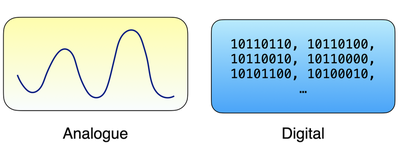
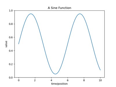
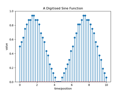
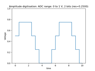
Computers are digital systems and and at he most basic level store information as sequences of bits (electronic states representing a 0 or 1, for more information on voltages and logic levels see here). Since there are only a finite number of ways of arranging a number of bits, digital numbers are thus restricted to finite range of values. Similarly, computer memory is finite and so is the number of digital values which can be stored. Thus, a signal stored on a computer is discrete in both value (amplitide) and time, as illustrated in the two figures below:
In the real world, analogue signals are continuous in both time and amplitude, and interfacing with a computer involves conversion between the digital and analogue domains. This ultimately involves either or both of:
- sending a digital number from the computer to a device which converts it into an analogue signal
or
- taking an analogue signal and converting it into a digital signal which is sent to the computer.
The common nomenclature is:
| Term | Acronym | Meaning |
|---|---|---|
| Digitial-to-Analogue Converter | DAC | Takes a digital signal (from computer) and convert to an analogue output signal |
| Analogue-Digital Converter | ADC | Converts an analogue signal to digital for recording by the computer |
In addition, sometimes digital signals are sent directy to control devices which have on/off states or to provide ‘clock’ signals for example to move stepper motors.
Bits, Bytes and Binary Numbers
Internally computers manipulate bits, which are voltages that represent either a ‘1’ or a ‘0’. Individual bits are grouped together to store information (a collection of 8 bits is called a ‘byte’). For examples, ADCs may be 8 bit, 12 bit, 16 bit etc. The bits when combined form a binary number since each location has only two possible values.
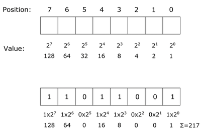
For example, consider a byte consisting of 8 bits as shown below. Each bit has a weight based on its position; the lowest weight (“least significant bit”) is on the right and the weights double with each place to the left since each position can have two possibilities (a 1 or 0). The number of possible values is given by 28=256 (0 to 255)
Binary in Python
Please see the secion in Python on binary numbers… (link to be added)
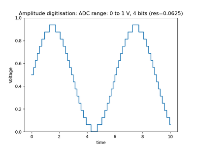
Digitisation and Amplitude Resolution
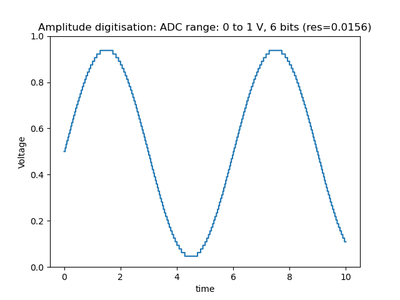
Since computers only store digital values digitised values are discrete. The number of bits combined with the range of the ADC or DAC determines the resolution. For example, an 8-bit ADC with a range of 5V has a resolution of ~0.0195V (5V/256) while a 12-bit ADC with a range of 5V has a resolution of 0.0012V (5V/4096). The affect of the number of bits on the amplitude resolution can be seen in the figures below:
Digitisation and Sampling
As mentioned above, due to the discrete nature of computers, signals which change are only captured at discrete instances. The process of digisiting a signal as discrete intervals is known as sampling. Sampling can introduce artefacts into digitised signals and it is critical to understand the basics of sampling theory.
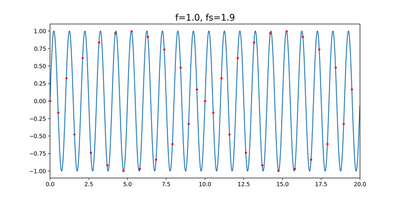
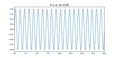
How many samples are needed to adequately describe a signal? The animation below illustrates what happens when a signal is sampled at different rates (note in the caption ‘f’ is the frequency of the signal and ‘fs’ is the sampling frequency):
As can be seen signals of the wrong frequencies appear (aliasing) when the sample rate drops to less than twice the frequency of the signal.
The Nyquist Sampling Criterion
The Nyquist Sampling Theorem states that to completely record all of the information in a signal it must be sampled at at least twice the highest frequency present, otherwise aliasing (the artifical transfer of power to lower frequencies occurs). For a perfect sine wave this may also be states as a minimum of two points per cycle.
A remarkable fact about the Nyquist sampling theorem is than once you have met the sampling criterion, all of the information about the original signal is captured in the samples and the the original signal can be completely reconstructed from the them. This has many applications in science, engineering, telecommunications etc. and, for example, why CD players use 44,100 Hz sampling
Aliasing is one of the reasons wheels can appear to rotate backward, see e.g. link and link